Basic plotting of geospatial data¶

# Ensuring high resolution plots from mac device
%config InlineBackend.figure_format = 'retina'

Plotting vector data¶

Vector data are data represented by a series of vertices, sometimes connected by edges. You typically have 4 types:

Points. Single vertices (e.g. a latitude and longitude coordinate pair that represents the location of an ATM machine)
Lines. Sets of vertices that are connected by edges (e.g. 3 latitude/longitude pairs that define the location of a road).
Polygons. Sets of vertices connected by edges where the last vertex and the first vertex are the same (e.g. 4 latitude/longitude pairs that define the outline of a building)
Multi-polygons. A collection of polygons (e.g. a university represented as a collection of polygon buildings or a building with an inner courtyard defined by an outer and inner polygon)

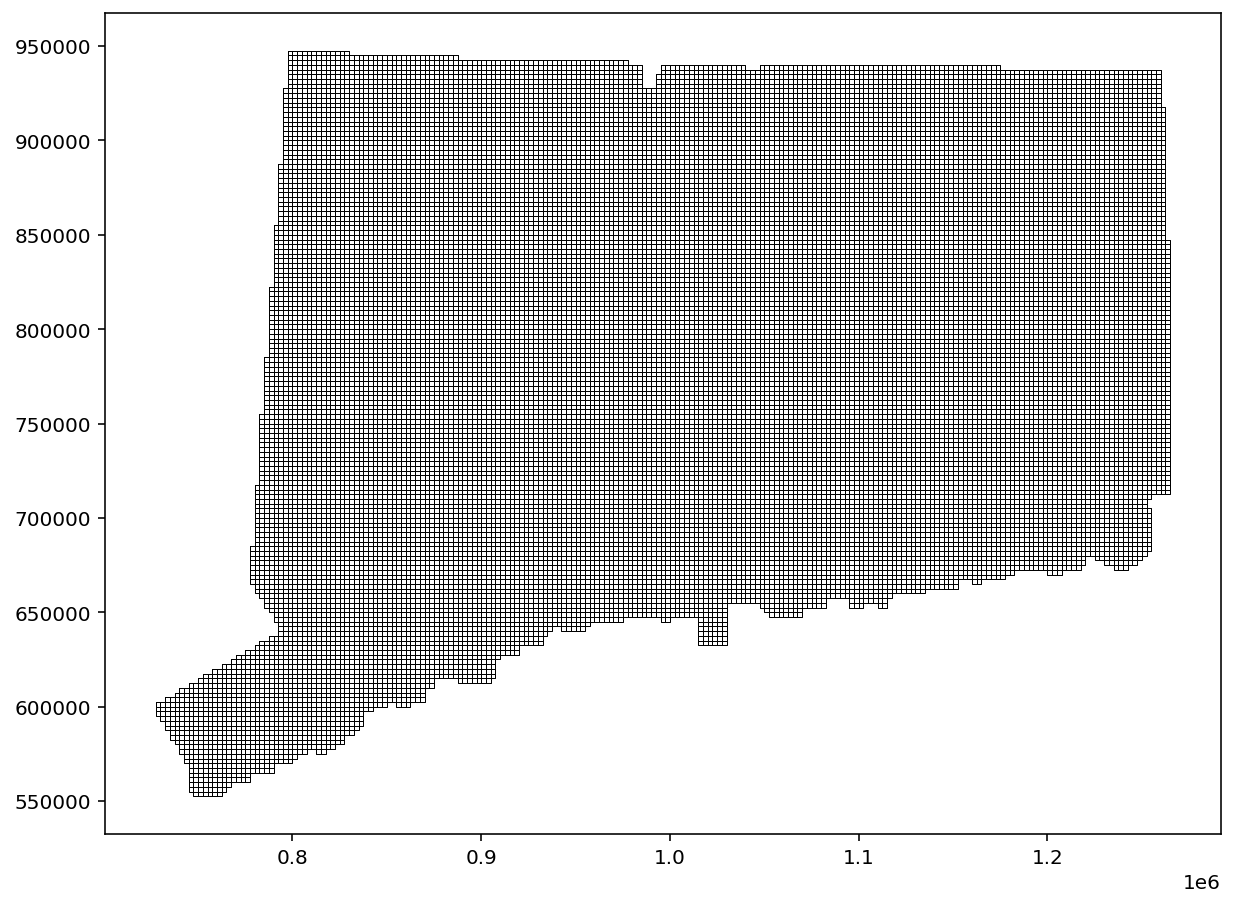
In this example, we’ll start by walking through how to plotpolygons representing a grid accross the state of Connecticut.

import numpy as np
import matplotlib as mpl
import matplotlib.pyplot as plt
import geopandas as gpd
import rasterio
from rasterio.plot import show
from rasterio.features import rasterize

plt.close('all')

fig, ax = plt.subplots(num='main', figsize=(10,10))

data_path = "./data/DeliveryGrid2016/DeliveryGrid.shp"

# Plot the grid of all tiles in Connecticut
full_data = gpd.read_file(data_path)
ctgrid = full_data.to_crs(epsg=6434).copy()
ctgrid.plot(ax=ax, color='none', linewidth=0.5, edgecolor='black')

<AxesSubplot:>

fig, ax = plt.subplots(num='main', figsize=(6,6))

# %%
# Plot the image transforming the coordinates from pixel coordinates to EPSG6434 coordinates
# data = rasterio.open('data/images/180700_se.tif')
# show(data.read([1,2,3]).astype('float')/65536, transform=data.transform, ax=ax)
data = rasterio.open('data/images/cropped.tif')
show(data.read([1,2,3]).astype('float')/255, transform=data.transform, ax=ax)

# %%
# PLOT SEGMENTATION DATA
raw_segmentation = gpd.read_file("data/annotations/segmentation.geojson")
segmentation = raw_segmentation.to_crs(epsg=6434).copy()
segmentation = segmentation.assign(label=0) # Sets default label to 0
# Convert Other, TP, FP, and FN to numerical values
for (i, entry) in enumerate(segmentation.iterrows()):
    if entry[1].default == 'TP':
        segmentation.at[i,'label'] = 1
    elif entry[1].default == 'FP':
        segmentation.at[i,'label'] = 2
    elif entry[1].default == 'FN':
        segmentation.at[i,'label'] = 3
# segmentation.plot(ax=ax, linewidth=1, ec=(0,0,1,1), fc=(0,0,1,0.25))

# Need to feed in pairs of geometries and the corresponding values to use
shapes = []
for (i, entry) in enumerate(segmentation.iterrows()):
    shapes.append((segmentation.at[i,'geometry'], segmentation.at[i,'label']))


result = rasterize(shapes,out_shape=data.shape, transform=data.transform)
masked_labels = np.ma.masked_where(result == 0, result)
colors = [
          (0.01,0.91,0.04),
          (1,0,0),
          (1,0.78,0.2)]
cmap = mpl.colors.LinearSegmentedColormap.from_list(
    'Custom cmap', colors, N=len(colors))
show(masked_labels, transform=data.transform, ax=ax, alpha=0.4, cmap=cmap, interpolation='none')

ax.set_xticks([])
ax.set_yticks([])

# Plot manual annotations
raw_annotations = gpd.read_file("data/annotations/annotations.geojson")
annotations = raw_annotations.to_crs(epsg=6434).copy()
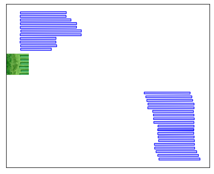
annotations.plot(ax=ax, linewidth=1, edgecolor=(0,0,1,1), facecolor=(0,0,1,0.25))

<AxesSubplot:>

Python for geospatial imagery

Basic plotting of geospatial data¶

Plotting vector data¶